🔎 Background
This project studies how to make fixed-point online learning stable when a deployed model must keep training after its input distribution changes.
The 🚂ENABOL paper frames the stability problem as a bounded-gain control problem. A trainable fixed-point network should not let activations, gradients, weights, or optimizer updates exceed the rails implied by the chosen ap_fixed formats. The proposed mechanism is kappa budgeting: assign per-layer induced-norm budgets and enforce them during training.
The very basics of neural networks
Let's start with the basics. We have some input data that defines some predictive features; and some output data that defines some observations; and we expect these two spaces to be related by some underlying function that we want to learn.
Then, we define a parametric model that we hope can approximate well for some choice of parameters . This is our neural network.
The question now is how do we tune to make a good approximation of ? The standard answer is to define a loss function that measures how well the model's predictions match the true outputs (according to some criterion of wellness), and then minimize the expected loss over the data distribution:
In practice, we usually don't have access to the true data distribution , so we work with a finite dataset and minimize the empirical loss:
The loss landscape
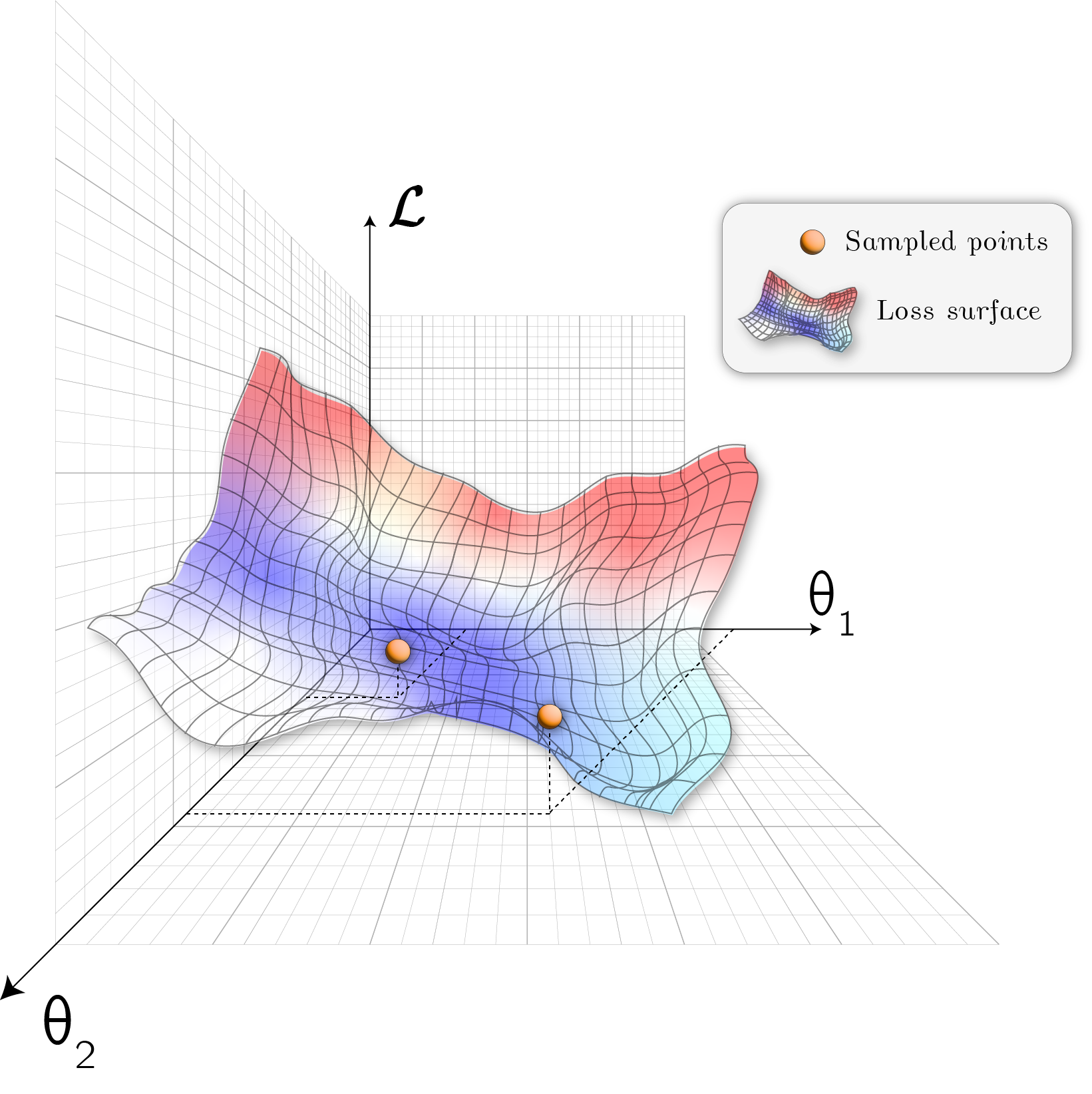
Now, the loss function and the model together define a landscape over the parameter space . What on earth does this mean? Imagine a very simple problem in which we only have two parameters , and the loss is a function of these two parameters. Because both and are deterministic, we know that for any combination of input value , output value and parameter values , the final loss will be a single static number.
This is important. Training, then, is just a process of sampling points in this loss landscape. We do not necessarily have access to the full landscape, nor we store it in memory, because doing so would be impossible for even moderately sized models (curse of dimensionality). So instead in regular stochastic training what we do is follow some local path through the landscape. But note that the important matter here is that the landscape itself is fixed. It does not change as we train. Parameters DO change, but the loss landscape itself is a static object that we are navigating through (as long as the loss function and model are deterministic, which is the case for our experiments).
Figure 1 shows an illustration of this. The 3D surface in this plot represents the loss landscape. The horizontal axes are the two parameters and , and the vertical axis is the loss value . The landscape has hills, valleys, and plateaus. The goal of training is to find a path through this landscape that leads us to a low-loss region, ideally a global minimum.
The gradient and curvature of the loss landscape
Since we are defining the loss as a function of fitness, we normally call training the process of following a certain path through the landscape such that we optimize this function (e.g., minimize the loss -as a definition of error- for a typical classification or regression problem). But what does it mean to follow a path through the landscape? How do we know which direction to go?
The most common answer is to use the gradient of the loss with respect to the parameters . This gradient is basically a vector field that tells us:
If I change the parameters by a small infinitesimal amount in some particular direction, how does the loss change?
Imagine that you are blindfolded and stopped at some point in a hilly landscape. This particular point where you are is defined by the current state of your model, i.e., the current parameters . Now, you want to find your way, say, downhill. What would you do? You would probably try to feel or probe the ground around you with your feet to see which direction is going down. This, my friend, is precisely what obtaining the gradient around that point means. The gradient is the local directionality of the loss landscape.
Mathematically, this gradient is defined as:
Gradient descent and the update rule
Once we have the gradient, we can use it to define an update rule for our parameters. The most basic one is the vanilla gradient descent update (also known Stochastic Gradient Descent or SGD when applied to mini-batches of data):
where is the learning rate, a hyperparameter that controls how big of a step we take in the direction of the negative gradient. What this rule is telling us is that the change in our parameters at step (mathematically, ) is proportional to the negative of the gradient at step .
In other words, in continuous time, this would be represented by something like:
which is a differential equation that describes how the parameters evolve over time under the influence of the gradient. Now, this is one of the easiest and most intuitive ODEs to solve, because it's simple and first order.
Given that is a positive constant, if we analyze its stability we see that this system will converge to a local minimum of the loss as long as is not too large. Why? Let's apply Lyapunov stability analysis to see why.
Lyapunov stability analysis on SGD
We want to find a Lyapunov function that can help us analyze the stability of the system. A natural choice for this function is the loss itself, . Now, we need to compute the time derivative of this Lyapunov function along the trajectories of the system. Using the chain rule (yes, the standard chain rule of calculus they teach you at school), we have:
Since is always non-negative, we have that for all . This means that the Lyapunov function is non-increasing along the trajectories of the system. Therefore, the system is stable in the sense of Lyapunov. Moreover, if the loss function is radially unbounded (i.e., as ), then we can conclude that the system is globally asymptotically stable, meaning that it will converge to a local minimum of the loss from any initial condition.
But what about the maximum value that we mentioned earlier? To find this, we can look at the curvature of the loss landscape, which is given by the Hessian matrix . The eigenvalues of this Hessian matrix tell us about the curvature in different directions. If the largest eigenvalue of the Hessian is , then we need to ensure that our learning rate is less than to guarantee convergence. This is because if is too large, we might overshoot and diverge instead of converging to a minimum.
Slow down. Where did this condition come from? Let's derive it step by step and very carefully. We will use another basic tool for this: Taylor expansion. First, recall the formula for Taylor series:
where is the -th derivative of evaluated at . Now, for any given point , let's approximate this loss function around up to second order:
But now, let's note something important:
- is precisely the gradient introduced before, and
- is precisely the Hessian , and
So we can rewrite the Taylor expansion as:
Now, let's analyze the stability of this system around some small perturbation around a local minimum . This means that we will set and . Substituting this into the Taylor expansion, we get:
Now, if we apply the gradient descent update rule, we have:
Let's define , where is a local minimum of the loss. Then, we can write:
Now, we can use the Taylor expansion of the loss around to express in terms of :
since at a local minimum. Substituting this back into the update for , we get:
Now, for the system to be stable, we need the spectral radius of the matrix to be less than 1. The spectral radius is the largest absolute value of the eigenvalues of this matrix. The eigenvalues of are given by , where are the eigenvalues of . Therefore, we need:
This leads to the condition:
sum to both sides, and this simplifies to:
Since is the largest eigenvalue, we need to ensure that , which gives us the final condition for convergence:
Why stop at the Hessian?
When analyzing stability we introduced an approximation around some point, via taylor expansion, but we stopped at second order (Hessian). But why not go further? We could, in principle. The reason why we don't is ... boring: the hessian is already too computationally expensive for us to compute, let alone higher-order derivatives.
In fact, we never even use Hessians in practice for our neural networks. Even modest-sized neural networks have millions of parameters, which means that computing the full Hessian matrix would require storing and manipulating a matrix with trillions of entries, which is completely infeasible. Instead, we often use approximations to the Hessian, such as the diagonal approximation used in algorithms like Adam, or we use techniques like stochastic estimation of the curvature.
The issue of online learning
Training a neural network on chip has many issues, but in this case we are going to focus on two:
- Quantization and fixed-point representation turns our problem into a non-trivial control problem because quantization introduces errors in the loss-landscape;
- The data distribution can change over time, which means that the loss landscape itself can change as we train.
Both of these problems, as you can see, are issues that, in the end, affect in the same way: they can change the training process in a way that can make the system unstable. The task of 🚂ENABOL is to design a controller that can keep the training process stable under these conditions.