💰 κ-budgeting formulation
The original κ-budgeting idea
Originally, in our paper, we proposed a static projection mechanism to enforce a per-layer gain constraint: the -budgeting mechanism. The idea is simple: in order to control the overall gain of the network, we enforce a per-layer gain constraint. For a purely linear network with layers and no activations (ReLU, etc.), the output is given by:
and the exact input-output gain is:
Using submultiplicativity of matrix norms:
So if we enforce:
then:
The original static budgeting idea proposed that ensuring each layer's gain below a certain threshold would guarantee that the overall network gain is below the product of the per-layer budgets. We hypothesized that this would be sufficient to ensure stable training.
Breaking down into row/column budgets
In practice, we realized that the per-layer gain constraint affected to different paths/loops in which instability could emerge:
- the forward pass gain (which controls the activations and representational Lipschitzness),
- the backward pass gain (which controls the gradients).
In other words, due to the fix point precision quantization that hardware requires, we need to ensure that neither the gradients nor the activations explode (saturate) or vanish (underflow). This led us to break down the per-layer gain constraint into row and column budgets, which are more fine-grained and can control the gain in both directions.
This is where the and budgets come from: controls the maximum row norm (forward gain), while controls the maximum column norm (backward gain). Mathematically:
The actual implementation of this worked more or less like this:
- input W, gradients, η, κ_col_log2, κ_row_log2
- # Column budget: backward gradient gain
- for each input column i:
- col_sum ← sum_j |W[i,j]|
- col_shift ← max(0, ceil_log2(col_sum) - κ_col_log2)
- g_x[i] ← right_shift_round_sat(g_x_raw[i], col_shift)
- end for
- # Row throttle: Adam update gain
- for each output row j:
- row_sum ← sum_i |W[i,j]|
- grad_sum ← sum_i |gW[i,j]|
- update_shift ← max(0, ceil_log2(row_sum) + ceil_log2(η) + ceil_log2(grad_sum) - κ_row_log2)
- apply Adam update with update step right-shifted by update_shift
- end for
- # Row budget: post-update weight projection
- for each output row j:
- row_sum ← sum_i |W[i,j]|
- row_shift ← max(0, ceil_log2(row_sum) - κ_row_log2)
- W[:,j] ← right_shift_round_sat(W[:,j], row_shift)
- end for
The actual code in cpp, for example for nnet_dense_backpass.h, looks like this for the row scaling part:
RowScale:
  {
    for (int j = 0; j < C_out; ++j) {
      #pragma HLS PIPELINE II=1

      // 1) exponent of current row L1
      ap_int<16> e_row = autograd::ceil_log2_fixed(l1_row[j]);  // sentinel −32768 if 0
      if (e_row == ap_int<16>(-32768)) continue;                // zero row ⇒ nothing to do

      // 2) κ_row exponent MUST be ceil(log2 κ_row) from the config generator
      const ap_int<16> E_ROW_CAP = (ap_int<16>)kappa_row_log2;  // this is ⌈log2 κ_row⌉

      // 3) hysteresis (optional): require at least HYS extra exponent before clamping
      //    set CONFIG_T::kappa_row_hys_bits = 0 or 1 (default 0 if not provided)
      const int HYS = 1; //(int)CONFIG_T::kappa_row_hys_bits;        // e.g., 0 or 1
      ap_int<16> e_diff = e_row - E_ROW_CAP;

      // k = max(0, e_diff - HYS)
      ap_uint<16> k = (e_diff > HYS) ? (ap_uint<16>)(e_diff - HYS) : (ap_uint<16>)0;
      scale_row[j] = k;

      // 4) Apply scaling if needed
      if (k != 0) {
        // Project the row by 2^{-k} (power-of-two L1 projection)
        ScaleRow:
        {
          for (int i = 0; i < C_in; ++i) {
            const int idx = i * C_out + j;
            // widen → shift with rounding/sat → cast back
            weight_accum_t w_wide = (weight_accum_t)weights[idx];
            w_wide = autograd::rshift_round_sat(w_wide, k);
            weights[idx] = (weight_t)w_wide;
          } // for i
        } // ScaleRow
      } // if k != 0
    } // for j
  } // RowScale.
While the column scaling part inside the optimizer was mainly used as throttling (e.g., optimizers.h):
// Weights
WeightsRow:
{
  for (int j = 0; j < C_out; ++j) {
    #pragma HLS PIPELINE II=1
    ap_uint<16> s = s_row[j];

    for (int i = 0; i < C_in; ++i) {
      const int idx = i * C_out + j;

      // grads
      uW_t g = (uW_t)gW_avg[idx];

      // m, v updates
      mW[idx] = (mW_t)( beta1 * (mW_t)mW[idx] + (one - beta1) * (mW_t)g );
      // square in widened type to avoid overflow; cast back
      uW_t g2 = (uW_t)g * (uW_t)g;
      vW[idx] = (vW_t)( beta2 * (vW_t)vW[idx] + (one - beta2) * (vW_t)g2 );


      // bias correction ≈ multiply by scalar factors
      // b1t = 1 - beta1^t ; b2t = 1 - beta2^t
      double b1t = 1.0, b2t = 1.0;
      // cheap pow via double; replace with LUT if you want pure fixed
      b1t -= std::pow((double)beta1, (int)t);
      b2t -= std::pow((double)beta2, (int)t);
      opt_scalar_t ib1 = (opt_scalar_t)(1.0 / b1t);
      opt_scalar_t ib2 = (opt_scalar_t)(1.0 / b2t);

      uW_t mhat = (uW_t)((opt_scalar_t)mW[idx] * ib1);
      uW_t vhat = (uW_t)((opt_scalar_t)vW[idx] * ib2);


      // denom = sqrt(vhat) + eps  => use rsqrt and multiply
      uW_t inv_s = rsqrt_safe<uW_t>(vhat, eps);
      uW_t step  = (uW_t)((opt_scalar_t)mhat * (opt_scalar_t)inv_s); // mhat / sqrt(vhat+eps)

      // throttle the step (shift)
      uW_t step_th = rshift_round_sat(step, s);

      // apply lr
      uW_t delta = (uW_t)lr * step_th;

      // update
      W[idx] = (typename CONFIG_T::weight_t)( (uW_t)W[idx] - delta );
    } // for i
  } // for j
} // WeightsRow.
❌ Why κ row/col failed
In our initial experiments, we found that we had to disable -row projection (RowScale{} block) to get any meaningful learning. But why??
The problem is that online learning is not only about whether the weights are inside a norm box. It is about the direction in parameter space. If the unconstrained gradient update is:
where:
- is the flattened vector of all trainable parameters,
- is the gradient,
- is the learning rate,
then the ideal update direction is:
But with row/column projection, the actual update becomes:
so the actual applied update is:
where is the projection caused by the constraint. This is generally not parallel to the gradient direction.
The row/column projection was enforcing that our gradients and our activations were constrained in norm, yes, but:
everytime we projected the weights using the , the direction of learning changed!
This means that the geometry of the landscape was not being preserved. The optimizer was trying to go downhill, but the projection was pushing it in a different direction.
What's worse, the projection was only being applied to the weights, but the gradients that each layer propagated to the rest of the backpass flow were not. This means that the actual change in weights at every layer was different than what the gradient was telling each layer up the stack to do. This is a fundamental mismatch between the geometry of the landscape and the actual trajectory that the optimizer was taking.
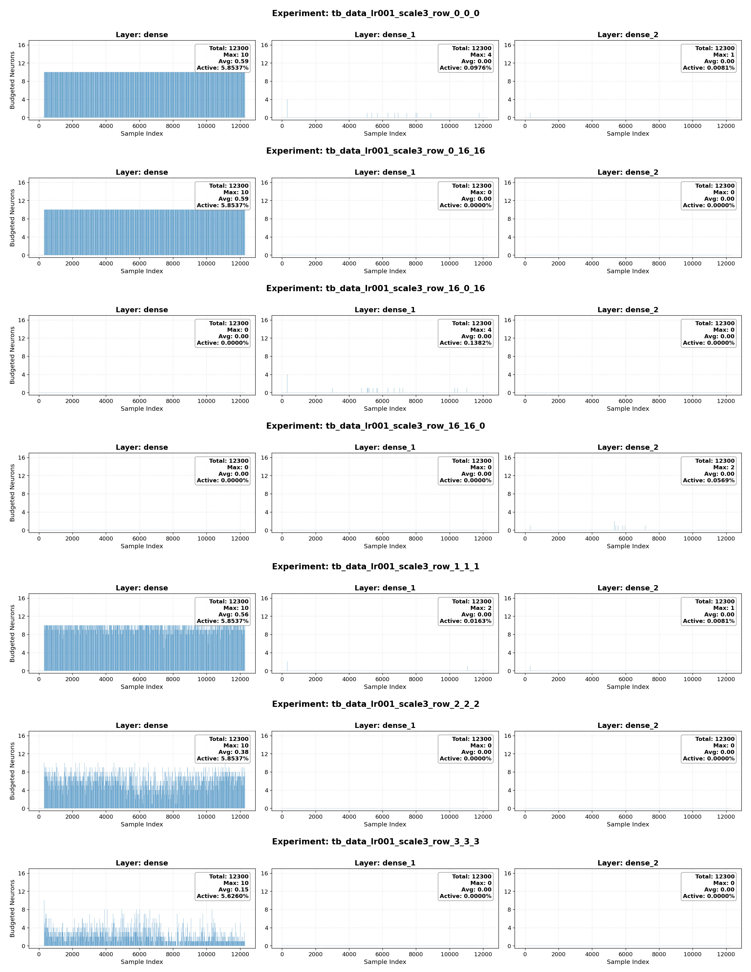
This becomes very clear with the tests that @Alan Guo ran. See the results below in Figure 2. In this experiment, the RowScale block was commented out, so the row projection was disabled. However, the column scaling (throttling) was still active. Here we show the frequency of throttling (and value), per training step, per layer (each column in this plot is a layer). The title of each group of panels shows the budget for each layer (e.g., the first one is ...row_0_0_0 meaning all three layers have the same col budget of .) The fact that the scaling applied to different layers is different means that the direction of learning is not being preserved.