DS-AFFINE-LINEAR-000: One-Layer Linear Teacher
Summary
This is the baseline synthetic regression dataset for the first global-throttle ablations. It is intentionally simple so the Hessian and stability boundary are analytically interpretable.
| Field | Value |
|---|---|
| Dataset ID | DS-AFFINE-LINEAR-000 |
| Family | Affine / linear teacher |
| Task | Regression |
| Input dimension | d_in = 4 |
| Output dimension | d_out = 2 |
| Bias | Disabled |
| Default samples | N = 1000 |
| Default drift | x_drift = gamma x, with gamma = 4 in EXP-000A and EXP-000B |
Generation
Inputs are sampled as:
Targets are generated by:
The default teacher matrix is:
So:
Code to generate the dataset:
If you need to understand the structure of this dataset, check here.
import enabol
# Create the dataset
dataset = enabol.AffineDataset(num_samples=1000, use_bias=False)
# Plot it
dataset.plot()
dataset.plot_histogram()
print(dataset)

# Get the data
X, Y = dataset.get()
which renders:
AffineDataset(
[Input] X:
  Shape: (1000, 4)
  Dtype: DataType.D2_FLOAT
  X <- Uniform(-1, 1)
[Output] Y:
  Shape: (1000, 2)
  Dtype: DataType.D2_FLOAT
  Y <- X @ A.T + b
---------------------------------
A = [[ 1.25 -0.75  0.5   0.2 ]
     [-0.4   0.9   1.1  -0.6 ]]
b = [0. 0.]
---------------------------------
Analytic Hessian:
  Lambda max: 1.0841
  Eta max: 1.8448
)
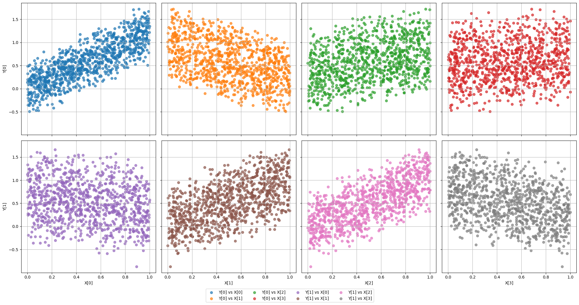
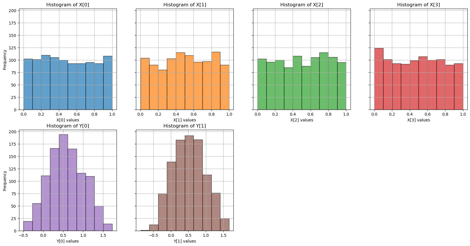
The following image shows scatter plots of the input and target distributions, as well as their histograms at the bottom.
Drift Model
The first drift model is pure input-gain drift:
For the first ablations:
The target remains consistent with the drifted input:
This isolates curvature-driven closed-loop instability without changing the underlying teacher rule.
Why This Dataset Exists
For one-layer no-bias linear regression, the loss is quadratic and the Hessian is tied to the input covariance. If the input is scaled by gamma, the dominant curvature grows approximately as:
That makes this dataset useful for checking whether a controller reacts coherently when a learning rate that was stable before drift becomes unstable after drift.
Used By
| Experiment | Role |
|---|---|
| EXP-000A | Float global-throttle sanity check. |
| EXP-000B | Quantized global-throttle sanity check. |
Implementation
Implemented by AffineDataset in the dataset module.
Reference: Dataset implementation